style> .boxes{width:50%;float:left;} #mainDiv{width:100%;margin:auto;} img{max-width:100%;}

FastS : Adaptive simulation of a supersonic flow around a diamond


The example shown here is the same case shown here: diamond IBM workflow.
The corresponding tutorial is described here: adaptive IBM workflow tutorial.

Adaptive mesh

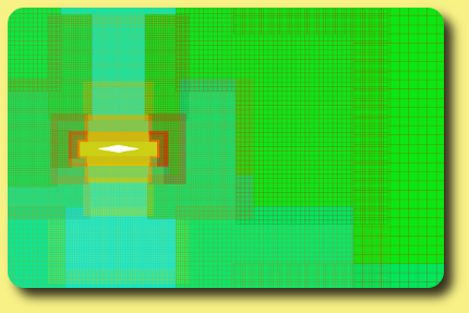
Adaptive mesh on a supersonic (Minf=2) inviscid flow simulation.
Sensor for adaptation: the difference of the Mach number. All the adaptations use a factor of 1.2 and do not add a refinement level, except for the last one, for which a refinement level is added and a factor of 1.5.

Initial mesh (snear=0.0058). 47 grids, 84 000 cells.
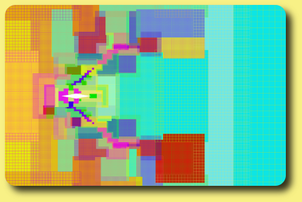

Mesh after 5 adaptations (snear=0.0029). 169 grids, 234 000 cells.


Mach number contours

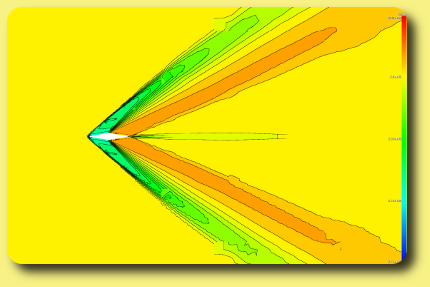
A view of the Mach number contours computed for the first and fifth meshes is displayed.

Initial Mach number field (snear=0.0058). 47 grids, 84 000 cells.
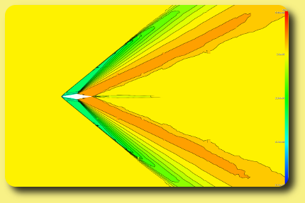

Mach number after 5 adaptations (snear=0.0029). 169 grids, 234 000 cells.


Sensor field

The sensor field, which is the difference of the Mach number here to capture the shocks, is displayed at the end of the first and fifth computations:
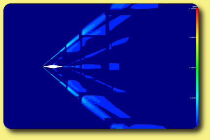
Initial sensor field (snear=0.0058). 47 grids, 84 000 cells.
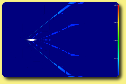

Sensor field after 5 adaptations (snear=0.0029). 169 grids, 234 000 cells.

                   
More: Gallery - Tutorials - Help forum - Index